This iPython notebook is an implementation of a popular paper (Gatys et al., 2015) that demonstrates how to use neural networks to transfer artistic style from one image onto another.

The implementation is slightly modified to use Densenet instead of VGG-Net and an additional regularization term is also added to the overall loss function.

The main objective of the algorithm is to merge two images, namely content image (C) and style image (S) to create a generated image (G) , which combines the content of the image C with the style of the image S.

For example, we can see the stylized image from the Taj Mahal (content image C), mixed with a painting by Van Gogh (style image S).

style_transfer_img1

The algorithm uses neural representations which are obtained by using Convolution Neural Networks (CNN), which are most powerful in image processing tasks. A CNN consists of a number of convolutional and subsampling layers optionally followed by fully connected layers, where each layer can be understood as a collection of image filters, each of which extracts a certain feature from the input image also called as feature maps.

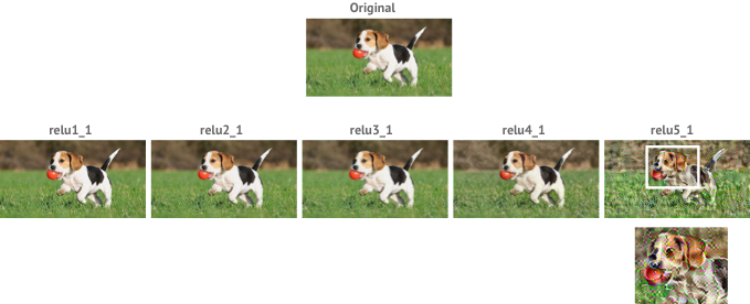
On training CNN for object recognition, along the processing hierarchy of the network, the feature maps represents more actual content of the image compared to its detailed pixel values. This can be visualized by reconstructing the image only from feature maps. This is called content reconstruction.

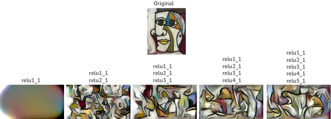
By including the feature correlations of multiple layers, we obtain a style representation of the input image, which captures its texture information but not the global arrangement. This representation captures general appearance in terms of colour and localised structures. This can be visualized by reconstructiing the image from feature maps showing texture information. This is called style reconstruction.

Key notes from the paper

Algorithm details & loss functions

Modifications to the approach

Implementation of the artistic style transfer algorithm

Load and preprocess the content and style images

Then, we convert these images into a form suitable for numerical processing. In particular, we add another dimension (beyond the classic height x width x 3 dimensions) so that we can later concatenate the representations of these two images into a common data structure.

Now we're ready to use these arrays to define variables in Keras' backend (the TensorFlow graph). We also introduce a placeholder variable to store the combination image (generated image) that retains the content of the content image while incorporating the style of the style image.

Finally, we concatenate all this image data into a single tensor that's suitable for processing by Keras' DenseNet121 model.

Reuse a model pre-trained for image classification to define loss functions

The core idea introduced by Gatys et al. (2015) is that convolutional neural networks (CNNs) pre-trained for image classification already know how to encode perceptual and semantic information about images. We're going to follow their idea, and use the feature spaces provided by one such model to independently work with content and style of images.

The original paper uses the 19 layer VGG network model from Simonyan and Zisserman (2015), but we're going to instead use DenseNet121 model.

Also, since we're not interested in the classification problem, we don't need the fully connected layers or the final softmax classifier. We only need the part of the model before "Classification Layer" from below architectures:

DenseNet Network Architectures

As seen above, for DenseNet-121 there are 121 layers (1 right after Input Layer, 116 from Dense Block, 3 from Transition Layer & 1 FC Layer). Note: Pooling is not considered as a layer.

It is trivial for us to get access to this truncated model because Keras comes with a set of pretrained models, including the DenseNet121 model we're interested in. Note that by setting include_top=False in the code below, we don't include any of the fully connected layers.

As it is clear from the table above, the model we're working with has a lot of layers. Keras has its own names for these layers. Let's make a list of these names so that we can easily refer to individual layers later.

If you stare at the list above, you'll convince yourself that we covered all items we wanted in the table. Notice also that because we provided Keras with a concrete input tensor, the various TensorFlow tensors get well-defined shapes.


The crux of the paper we're trying to reproduce is that the style transfer problem can be posed as an optimisation problem, where the loss function we want to minimise can be decomposed into three distinct parts: the content loss, the style loss and the total variation loss.

The content loss

The content loss is the (scaled, squared) Euclidean distance between feature representations of the content and combination images.

Selecting layer for content representation

For the content loss, we see that in Gatys et al. (2015) the choice of layer is made based on the ability of the feature-map to reconstruct image which preserves the high-level content of the original image but loses the exact pixel information.

For example: content_image_layer

The style loss

This is where things start to get a bit intricate.

For the style loss, we first define something called a Gram matrix. The terms of this matrix are proportional to the covariances of corresponding sets of features, and thus captures information about which features tend to activate together. By only capturing these aggregate statistics across the image, they are blind to the specific arrangement of objects inside the image. This is what allows them to capture information about style independent of content. (This is not trivial at all, and I refer you to a paper that attempts to explain the idea.)

The Gram matrix can be computed efficiently by reshaping the feature spaces suitably and taking an outer product.

The style loss is then the (scaled, squared) Frobenius norm of the difference between the Gram matrices of the style and combination images.

Selecting layers for style representation

For style loss, we see that in Gatys et al. (2015) they select layers which reconstructs images that match the style of a given image on an increasing scale while discarding information of the global arrangement of the scene.

For example:

style_image_representation

Note: As it can be seen in above reconstructed style image that the texture is not yet fully concise and hence the output combination image is not that of good quality as compared to the results in original paper.

The total variation loss

Now we're back on simpler ground.

If you were to solve the optimisation problem with only the two loss terms we've introduced so far (style and content), you'll find that the output is quite noisy. We thus add another term, called the total variation loss (a regularisation term) that encourages spatial smoothness.

You can experiment with reducing the total_variation_weight and play with the noise-level of the generated image.

Total variation loss works as regularizer for smoothing the generated image.

Final loss calculation

We'll now use the feature spaces provided by specific layers of our model to define these three loss functions:

The relative importance of loss terms are determined by a set of scalar weights. These are arbitrary, but the following set have been chosen after quite a bit of experimentation to find a set that generates output that's aesthetically pleasing to me.

Define needed gradients and solve the optimisation problem

The goal of this journey was to setup an optimisation problem that aims to solve for a combination image that contains the content of the content image, while having the style of the style image. Now that we have our input images massaged and our loss function calculators in place, all we have left to do is define gradients of the total loss relative to the combination image, and use these gradients to iteratively improve upon our combination image to minimise the loss.

We start by defining the gradients.

Now we're finally ready to solve our optimisation problem. This combination image begins its life as a random collection of (valid) pixels, and we use the L-BFGS algorithm (a quasi-Newton algorithm that's significantly quicker to converge than standard gradient descent) to iteratively improve upon it.

We stop after 80 iterations because the output looks good to me and the loss stops reducing significantly.

Overall code

Conclusion and further improvements

Compartive Studies

Perceptual Losses for Real-Time Style Transfer and Super-Resolution by Johnson et al., 2016

perceptual_loss_style_transfer

Universal Style Transfer via Feature Transforms by Li et al., 2017

References

  1. A neural algorithm of artistic style (2015) - Leon A. Gatys, Alexander S. Ecker, Matthias Bethge
  2. Densely Connected Convolutional Networks - Gao Huang, Zhuang Liu, Laurens van der Maaten, Kilian Q. Weinberger
  3. Perceptual Losses for Real-Time Style Transfer and Super-Resolution - Justin Johnson, Alexandre Alahi, Li Fei-Fei
  4. Artistic style transfer implementation with a repurposed VGG-Net-16 - H. Narayanan
  5. Fast Neural Style - Code - Justin Johnson et al.
  6. Universal Style Transfer via Feature Transforms - Li et al.
  7. Tensorflow/Keras implementation of WCT
  8. iPython Notebook of this post